Diffusion Models for Language
Graham Neubig
What is Diffusion?
Forward Process
Gradually add noise to data over multiple timesteps

Reverse Process
Learn to denoise, going from noise back to data

Practical Examples in Language Generation
Mathematical Framework
Given a datum that we would like to model \(x_0 \sim p_{\text{data}}(x)\)
- Forward Process: Add noise to data over \(T\) timesteps
with noising function \(q(x_t \mid x_{t-1})\)
- Typically simple (e.g. Gaussian noise for images)
- Reverse Process: Learn a probability distribution to denoise data
\(p_\theta(x_{t-1} \mid x_t)\)
- Typically a neural network with parameters \(\theta\)
Denoising Diffusion Probabilistic Models (DDPM)
Reference: Ho et al., NeurIPS 2020

Forward Diffusion Process
Goal: Gradually destroy structure in data distribution over \(T\) timesteps
Given datum \(x_0 \sim p_{\text{data}}\), define forward process as Gaussian noise:
\(q(x_t \mid x_{t-1}) = \mathcal{N}(x_t; \sqrt{1-\beta_t} x_{t-1}, \beta_t I)\)
where \(\beta_1, ..., \beta_T\) is the variance schedule (how fast we add noise over time)
Efficiency Tricks
- Can jump directly to any noise level \(t\) without going step-by-step!
- Cumulative signal retention: Let \(\alpha_t = 1 - \beta_t\) and \(\bar{\alpha}_t = \prod_{s=1}^t \alpha_s\)
- We can propagate gradients through the reparameterization trick:
- \(x_t = \sqrt{\bar{\alpha}_t} x_0 + \sqrt{1-\bar{\alpha}_t} \epsilon\)
- where \(\epsilon \sim \mathcal{N}(0, I)\) is standard Gaussian noise
- \(\bar{\alpha}_t\) controls the signal-to-noise ratio at time \(t\)
Score Matching
- A score function points in the direction where we can increase probability
- \(s(x) = \nabla_x \log p(x)\) (gradient of log-probability)

(img credit: Song 2021)
Denoising Score Matching
Given clean data \(x_0\) and the noise \(\epsilon\), we know exactly what the score should be!
\(s_\theta(x_t,t) = -\frac{1}{\sigma_t},\epsilon_\theta(x_t,t)\)
Training objective: Train a neural network to predict the noise that was added
\(\mathcal{L}_{\text{DSM}} = \mathbb{E}_{x_0, \epsilon} \left[ \| \epsilon - \epsilon_\theta(x_t, t) \|^2 \right]\)
This is just MSE loss - predict the noise, minimize squared error
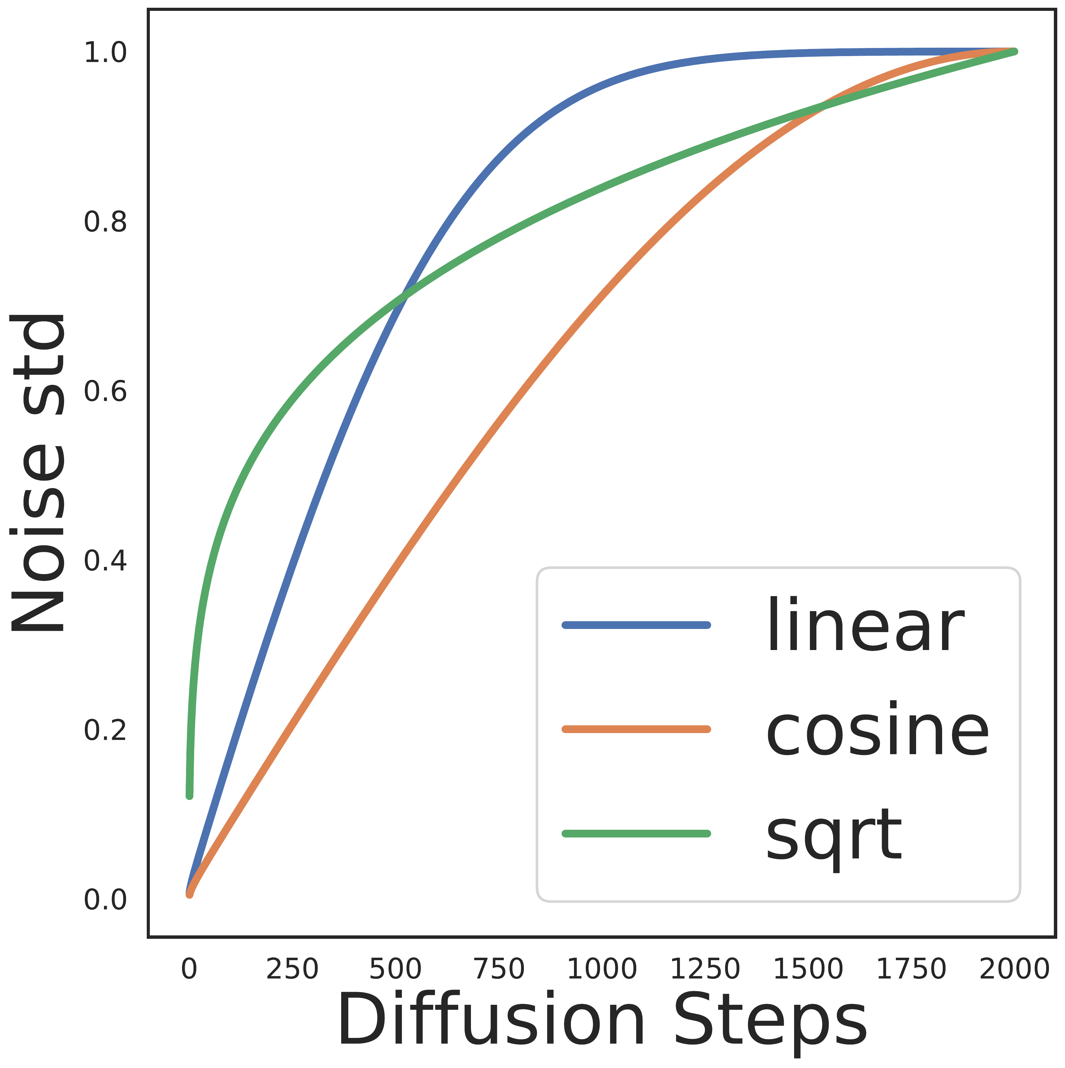
Noise Schedule Design
Variance Schedule: Controls rate of noise addition
- Linear: \(\beta_t = \beta_1 + \frac{t-1}{T-1}(\beta_T - \beta_1)\)
- Cosine: More gradual noise addition, better for details
Sampling Strategies
Stochastic Sampling:
\(x_{t-1} = \text{denoise}(x_t) + \sigma_t \epsilon\) where \(\epsilon \sim \mathcal{N}(0, I)\)
- More diverse outputs
- Explores different possible generations
Deterministic Search (Mode-seeking):
\(x_{t-1} = \text{denoise}(x_t)\)
- Faster generation (can skip steps)
- Less diverse outputs
DDPM Success on Images
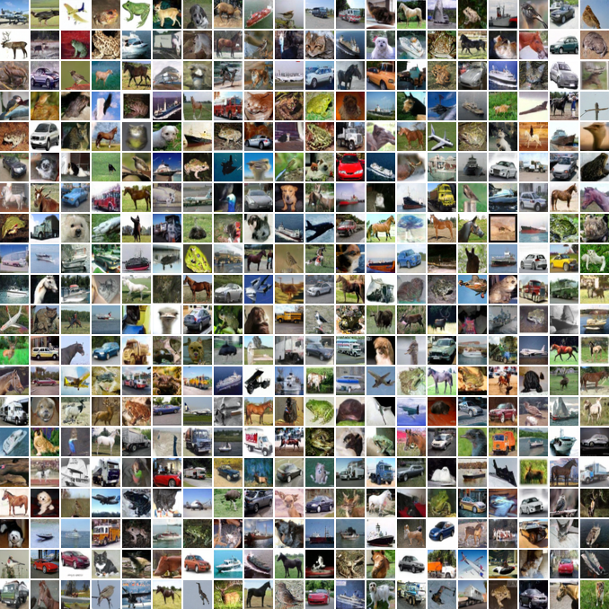
- FID 3.17 on CIFAR-10 (state-of-the-art at the time)
- High quality without adversarial training
- Stable training process
Progressive Generation in Images

Observation: Diffusion models generate coarse-to-fine
- Early steps: Overall structure, global features
- Middle steps: Local patterns, textures
- Late steps: Fine details, high-frequency information
Part 2: The Language Challenge
Why Can’t We Just Apply Image Diffusion to Text?
The Discrete Problem
Images are Continuous:
- Images are continuous-valued (pixels in [0, 1])
- Size is fixed (e.g., 32x32, 256x256)
Language is Discrete:
- Tokens from a discrete vocabulary
- Variable-length sequences
Two Approaches to Language Diffusion
1. Continuous Embeddings (Diffusion-LM)
- Map tokens to continuous space
- Apply diffusion in embedding space
- Round back to discrete tokens
2. Discrete Diffusion
- Define noise processes directly on discrete data
- Corruption operations: masking, replacement, edits
- Learn to reverse the corruption
- Example approaches: MDLM (masking), SEDD (score-based), Diffuser (edit-based)
Why Diffusion for Language?
- Potential Advantages:
- Non-autoregressive: Generate/edit all positions in parallel
- Flexible editing: Modify specific parts without full regeneration
- Controllability: Natural framework for constraints
- Iterative refinement: Multiple passes improve quality
- Current Reality:
- Autoregressive models still dominate in quality
- Diffusion offers unique capabilities for specific tasks
- Active area of research with rapid progress
Part 3: Solutions for Language
Continuous Approaches
Diffusion-LM: Continuous Embeddings
Reference: Li et al., NeurIPS 2022
Key Idea: Apply diffusion in continuous embedding space
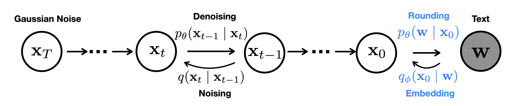
Diffusion-LM: The Approach
Process:
-
Embed: Map discrete tokens to continuous vectors \(\text{emb}(w) = E_w\) where \(E \in \mathbb{R}^{V \times d}\) is the embedding matrix, \(V\) is vocabulary size, \(d\) is embedding dimension
-
Diffuse: Add noise in embedding space \(x_t = \sqrt{\bar{\alpha}_t} \text{emb}(w) + \sqrt{1-\bar{\alpha}_t} \epsilon\)
-
Denoise: Learn to predict clean embeddings \(\epsilon_\theta(x_t, t) \approx \epsilon\)
-
Round: Map back to discrete tokens \(w' = \arg\max_w \cos(E_w, \hat{x}_0)\) where \(E_w\) is the embedding for word \(w\)
Challenge: Rounding is non-differentiable
Diffusion-LM: Technical Details
Key Innovation - \(x_0\) Parameterization:
Instead of predicting noise \(\epsilon\), directly predict clean embeddings \(x_0\) at every step
Why this matters:
- Significantly reduces rounding errors
- Forces model to commit to concrete embeddings
- Makes it easier to map back to discrete tokens
Diffusion-LM: The Clamping Trick
Problem: Even with \(x_0\) prediction, rounding errors accumulate during sampling
Solution - Clamping at Decode Time:
Standard sampling from predicted \(x_0\):
With clamping:
where \(\text{Clamp}(x) = \arg\max_{w \in V} \cos(E_w, x)\) (nearest embedding by cosine similarity)
Effect: Forces intermediate predictions to commit to valid word embeddings, making subsequent predictions more precise
Diffusion-LM: Controllable Generation
Diffusion-LM allows for constraints during generation via gradient-based control
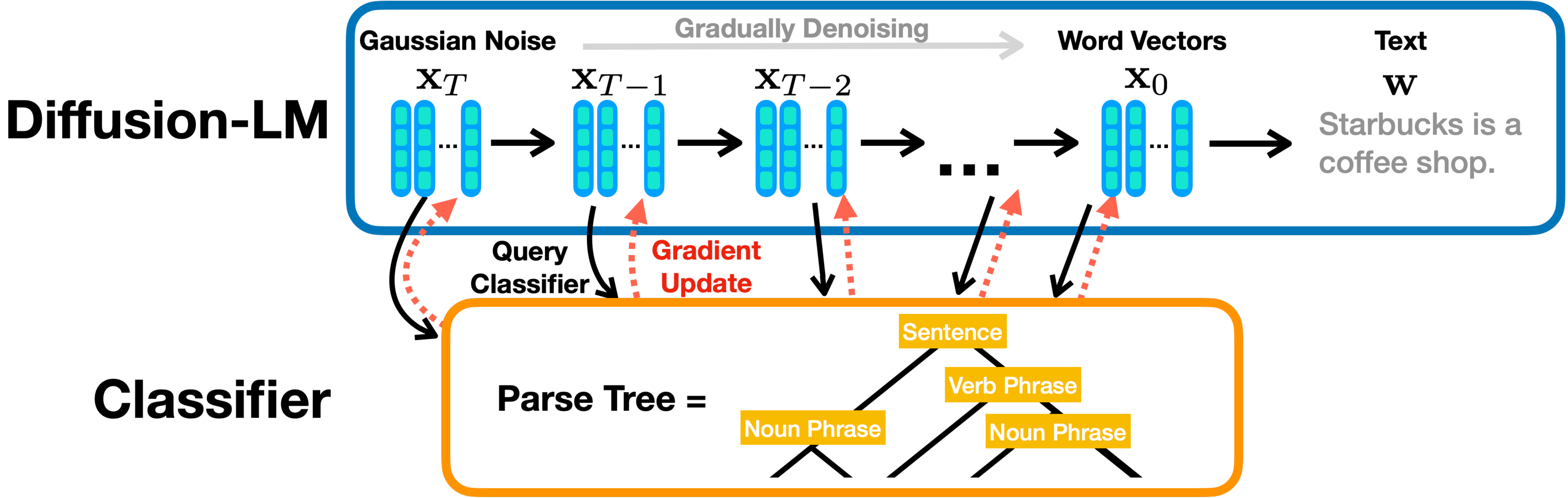
Diffusion-LM: Controllable Generation
Gradient-Based Control:
Modify denoising trajectory to satisfy constraints:
Example Controls:
- Syntactic Control: make output match a target parse tree
- Semantic Control: steer output towards a target sentiment or topic
- Length Control: enforce specific output length
Diffusion-LM: Results
- Higher perplexity (~36 vs. ~23 for GPT-2) but better controllability
- Controllability: Outperforms PPLM and FUDGE on 6 control tasks (syntax, semantics, infilling)
- Robustness: More resilient to local failures than autoregressive models (no exposure bias)
Weaknesses:
- Slower decoding (2000 diffusion steps vs. sequence-length AR steps)
- Slower training convergence than AR models
Part 3: Discrete Approaches
Working Directly with Discrete Data
Review: BERT and Masked Language Modeling
BERT (Bidirectional Encoder Representations from Transformers)
- Architecture: Encoder-only Transformer (bidirectional)
- Training: Masked Language Modeling (MLM)
Original:  The cat sat on the mat
Masked:    The [MASK] sat on the [MASK]
Predict:   "cat" and "mat"
- Not generative — can only fill in masked tokens, not generate from scratch
MDLM: Masked Diffusion Language Models
Reference: Sahoo et al., NeurIPS 2024
Key Innovation: Turns BERT-style masked LMs into generative models
Core Idea:
- Start with fully masked sequence:
[MASK] [MASK] [MASK] [MASK] - Gradually unmask tokens (reverse of gradually masking)
- Use BERT-like model to predict what tokens should be
Why it works:
- Training reduces to weighted masked language modeling - just like BERT with importance weights!
- Simple and stable training
- Can initialize from pretrained BERT models
MDLM: Forward Process
Forward Process: Gradually mask tokens
At time \(t\), randomly mask each token with probability \(m_t\):
$q(x_t \mid x_0) = \prod_i \begin{cases} \text{[MASK]} & \text{with probability } m_t \ x_{0,i} & \text{with probability } 1-m_t \end{cases}$
where \(m_t\) is the masking rate at timestep \(t\) (like a noise schedule)
Why masking?
- Natural corruption for text
- BERT-style MLMs already trained for this task
- Simpler than other discrete diffusion operations
MDLM: Training Objective
Training reduces to a weighted average of standard masked language modeling:
What this means:
- For each masked position \(i\), predict the original token
- Weight the loss by time-dependent factor \(w(t) = \frac{\alpha_t - \alpha_s}{1 - \alpha_t}\)
- Where \(\alpha_t\) is the cumulative unmasking rate at time \(t\)
- Comes from a theoretical lower bound on the likelihood
- That’s it - just like training BERT but with time-dependent importance weights!
MDLM: Inference 1 – Ancestral Sampling
- Start from fully masked sequence
- Iteratively unmask positions by sampling from \(p_\theta(x_0 \mid x_t, t)\)
- Random order: Unmasking happens stochastically based on the learned distribution
- No predetermined order - the model learns which positions to unmask when
- Continue until all positions are unmasked
MDLM: Inference 2 – Semi-Autoregressive Generation
- If we parameterize \(p_\theta(\cdot \mid x_t)\) without explicit time \(t\) (time-independent MDLM), we can cache logits for unmasked positions
- Why caching helps: Unmasked positions don’t change due to “carry-over unmasking” property
- Only recompute activations for newly unmasked positions at each step
- Cached positions remain unchanged throughout generation
- Extends naturally to variable-length sequences
- Efficient 2-3× speedup with caching
MDLM: Efficient Sampling with Caching
Problem: Recomputing all tokens at each step is wasteful
Solution: Cache activations for unchanged tokens
def sample_with_cache(model, x_t, cache):
    # Only compute changed positions
    changed_pos = get_masked_positions(x_t)
    new_activations = model(x_t, positions=changed_pos)

    # Reuse cached activations for unchanged positions
    cache.update(changed_pos, new_activations)

    # Predict and sample next state
    predictions = decode(cache.activations)
    return sample_next(predictions)
Speedup: 2-3× faster generation
MDLM: Results
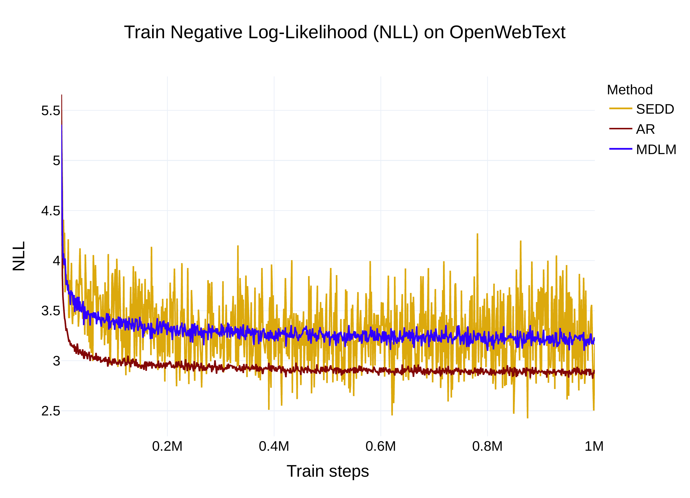
- New SOTA among diffusion LMs on multiple benchmarks
- Close to AR perplexity with good engineering
- Very simple and stable training (just weighted MLM)
- Perplexity on OpenWebText approaching AR baselines
SEDD: Score Entropy Discrete Diffusion
Reference: Lou et al., ICML 2024
Key Innovation: A principled score-based framework for discrete diffusion using continuous-time Markov chains
Core Idea:
- Models discrete diffusion as continuous-time Markov chain (CTMC)
- Learns probability ratios between tokens: \(s_\theta(x)_y \approx \frac{p(y)}{p(x)}\)
- Achieves better perplexity than GPT-2 - first discrete diffusion to do so!
SEDD: What Are Probability Ratios?
In continuous diffusion: Learn the score function \(\nabla_x \log p(x)\) (gradient pointing to higher probability)
In discrete diffusion: Can’t take gradients! Instead learn probability ratios:
What this means:
- For each position, learn relative likelihood of all possible tokens
- Not just “cat is correct” but “cat is 3× more likely than dog, 10× more likely than the”
- Richer signal than just predicting the correct token
Why ratios? They’re the discrete analog of the continuous score function
SEDD: Training with Score Entropy
Training objective: Learn to predict probability ratios via denoising
Score Entropy Loss:
What this does:
- Trains model to match true probability ratios from the forward process
- The ratios \(\frac{q(y|x_0)}{q(x_t|x_0)}\) are known from how we add noise!
- Squared error between predicted and true ratios
Key insight: Denoising makes this tractable - we know ground truth ratios
SEDD: Forward Process Design
Two transition designs for adding noise:
1. Uniform transitions:
# Each token can become any other token
Q_uniform[i,j] = 1/(V-1)  for i ≠ j
Q_uniform[i,i] = -1
2. Absorbing state (like MDLM):
# Tokens transition to [MASK], which absorbs
Q_absorb[i, MASK] = 1
Q_absorb[i, i] = -1
Q_absorb[MASK, MASK] = 0  # stays masked
Both parameterizations work - uniform is simpler, absorbing connects to MDLM
SEDD: Sampling via τ-leaping
Core idea: Take larger discrete steps, updating all positions in parallel
The update rule: At each position \(i\), sample new token from:
What this means:
- With probability \(\approx 1 - \Delta t\): stay at current token \(x_t^i\)
- With probability \(\propto \Delta t \cdot Q_t(x_t^i, y) \cdot s_\theta(\vec{x}_t)_{i,y}\): transition to token \(y\)
- The learned ratios \(s_\theta\) determine which transitions are more likely
Key property: All positions updated independently - enables parallel sampling
Tradeoff: Larger \(\Delta t\) = fewer steps but lower accuracy (like Euler discretization)
SEDD: Tweedie Denoising
Motivation: Can we do better than τ-leaping if we use the learned ratios more carefully?
Discrete Tweedie’s theorem: If we know all ratios \(\frac{p_t(y)}{p_t(x_t)}\), we can optimally denoise
Practical approximation: We only know ratios between nearby sequences, so:
- Estimate clean data: \(\hat{p}_0 = \exp(-\sigma_t^{\Delta t} Q) \cdot s_\theta(\vec{x}_t)\)
- Re-noise forward: Sample from \(\hat{p}_0\) re-noised to time \(t - \Delta t\)
The update rule: Sample token at position \(i\) from:
where \(\sigma_t^{\Delta t} = \overline{\sigma}(t) - \overline{\sigma}(t - \Delta t)\)
Benefit: Optimal among all parallel sampling strategies (proven in paper)
SEDD: Conditional Generation
Question: How to generate with constraints (e.g., fixed prefix, suffix, or infill)?
Key insight: Probability ratios make conditioning exact via Bayes’ rule:
What this means:
- \(\Omega\) = positions to generate (unfilled)
- \(\overline{\Omega}\) = positions to condition on (filled)
- Conditional ratios = unconditional ratios with fixed positions
In practice:
- Use the same model \(s_\theta\) trained unconditionally
- During sampling, only update positions in \(\Omega\)
- Keep positions in \(\overline{\Omega}\) fixed at their conditioned values
Examples: prefix continuation (\(\overline{\Omega} = \{1,...,c\}\)), suffix (\(\overline{\Omega} = \{d+1,...,n\}\)), infilling (any subset)
SEDD: Results
Perplexity Results (vs GPT-2 Small):
| Dataset | GPT-2 Small | SEDD | Improvement |
|---|---|---|---|
| LAMBADA | 45.04 | 42.77 | 5% better |
| WikiText2 | 42.43 | 31.04 | 27% better |
| PTB | 138.43 | 87.12 | 37% better |
| 1BW | 75.20 | 61.19 | 19% better |
Key Achievements:
- First discrete diffusion to beat autoregressive baselines
- 32× fewer function evaluations for comparable quality
- Principled likelihood-based training and evaluation
- Strong theoretical foundation (CTMC + score matching)
Diffuser: Edit-Based Reconstruction
Reference: Reid et al., arXiv 2022
Key Innovation: Uses all four Levenshtein edit operations for both corruption and reconstruction
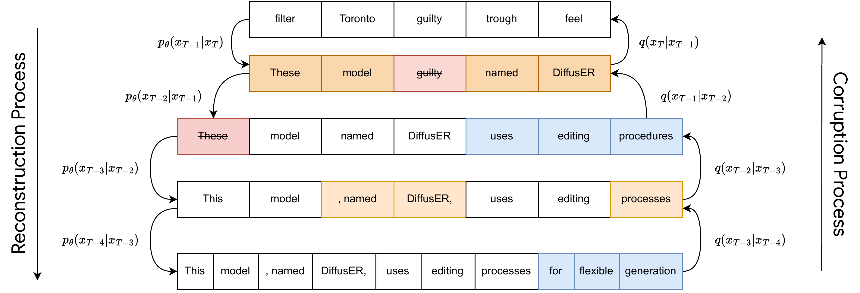
Core Idea:
- Models text generation as natural editing processes
- Uses INSERT, DELETE, KEEP, REPLACE operations
- Two-component architecture: tagger + generator
- Enables flexible editing in various contexts
Diffuser: Architecture
Two-Stage Process:
- Tagger: Predicts edit operations \(p^{\text{tag}}_\theta(e_t \mid x_t)\)
- Generator: Produces tokens for edits \(p^{\text{gen}}_\theta(x_{t-1} \mid x_t, e_t)\)
Edit Operations: INSERT, DELETE, REPLACE, KEEP
Training: Corrupt with reverse operations (e.g., train INSERT by adding deletions)
Corruption Parameters:
- \(E_t\): Edit type distribution (e.g., 60% keep, 20% replace, 10% delete, 10% insert)
- \(E_l\): Edit length distribution (e.g., Poisson λ=3)
Diffuser: Training Objectives
Both modules trained with cross-entropy losses:
Tagger Loss: Predicts edit operations
where \(e^*\) are the ground truth edit operations that generated \(x_t\) from \(x_{t-1}\)
Generator Loss: Predicts tokens at edited positions
Key Difference from Other Diffusion Models:
- Not using ELBO (Evidence Lower Bound) like DDPM/MDLM/SEDD
- Instead: Two separate supervised learning objectives
- Simpler training, but less theoretical grounding
- Leverages edit distance structure for natural editing workflow
Diffuser: Flexible Initialization
Bootstrap Strategies:
-
Null Sequence: Start from empty string
- First operation must be insertion
- Clean generation from scratch
-
Random Tokens: Start from random noise
- Model learns to edit random sequence into coherent text
- Similar to traditional diffusion
-
AR Bootstrap: Start from autoregressive model output
- Refine initial draft with diffusion
- Combines AR coherence with diffusion flexibility
-
Source Bootstrap: For seq2seq, start from source text
- Particularly effective for summarization
- Treats generation as editing task
Diffuser: 2D Beam Search
Novel Decoding Strategy:
Standard beam search only searches over tokens. Diffuser introduces 2D beam search:
- Intra-revision dimension: Beam width \(b\) for token-level search
- Inter-revision dimension: Beam width \(r\) for diffusion steps
Algorithm:
- Generate \(b\) candidates at current diffusion step
- Keep top \(r\) based on log-likelihood
- Feed all \(r\) to next diffusion step
- Each produces \(b\) new candidates → \(r \times b\) total
- Keep top \(r\) again
Result: Searches over both edit operations AND diffusion trajectories
Diffuser Results
Machine Translation (WMT’14 En-De):
| Method | BLEU |
|---|---|
| Autoregressive Transformer | 27.3 |
| Levenshtein Transformer | 23.7 |
| CMLM | 24.6 |
| Base Diffuser | 27.2 |
| Diffuser + AR Bootstrap | 28.8 |
| Diffuser + Source Bootstrap | 24.5 |
Summarization (CNN/DM):
| Method | ROUGE |
|---|---|
| Autoregressive | 36.8 |
| SUNDAE | 37.0 |
| Base Diffuser | 37.8 |
| Diffuser + AR Bootstrap | 38.4 |
| Diffuser + Source Bootstrap | 38.9 |
Key Findings:
- AR bootstrap best for translation (28.8 vs 27.3 baseline)
- Source bootstrap best for summarization (treats as editing)
- First non-AR model to beat AR on these tasks
Comparing Discrete Diffusion Approaches
| Method | Data Space | Forward Process | Training | Sampling | Key Strengths |
|---|---|---|---|---|---|
| Diffusion-LM | Continuous embeddings | Gaussian diffusion | Predict \(x_0\) + clamping | DDPM + rounding | Plug-and-play control via gradients |
| MDLM | Discrete (masking) | Time-dependent masking | Weighted MLM (Rao-Blackwell ELBO) | Ancestral unmasking + SAR | Simple, stable, new SOTA |
| SEDD | Discrete (CTMC) | Token transitions (\(Q_t\)) | Score entropy (ratio matching) | τ-leaping + Tweedie | Elegant, controllable, strong theory |
| Diffuser | Discrete (edits) | Levenshtein ops | Tagger + generator (CE losses) | 2D beam search | Best for editing/seq2seq tasks |